CDiD: Treatment Effects Beyond Complete Panels
A general toolkit for incomplete histories, staggered adoption, and selective observation
A firm enters a survey late. A household misses an interview. An administrative database records an outcome in some years but not others. In a rotating panel, every unit may be observed for only a short window. These are familiar features of applied research, yet restricting the analysis to units observed throughout can discard much of the data, change the population being studied, or leave no observations at all.
cdid estimates treatment effects by connecting the changes that are observed. Different units can supply different parts of the history. When those comparisons represent the same study population and satisfy the identifying assumptions, chaining them recovers effects over longer horizons.
Since the original introduction, the package has grown into a broader toolkit. It now brings together chained IPW, outcome regression, and doubly robust estimation; three corrections for covariate-dependent missing outcomes; alternative parallel-trends restrictions; and familiar tools for event studies and inference. Version 1.2.0.1 is available on CRAN.
The useful information is in the changes
The starting point is our paper with Christophe Bellégo and Vincent Dortet-Bernadet, The Chained Difference-in-Differences, published in the Journal of Econometrics in 2025. The package builds on the cohort and period treatment effects of Callaway and Sant’Anna (2021) and their did package.
Imagine treatment begins at date 3. One group of units is observed at dates 2 and 3, a second at dates 3 and 4, and a third at dates 4 and 5. No unit is observed at both the reference date 2 and the final date 5.
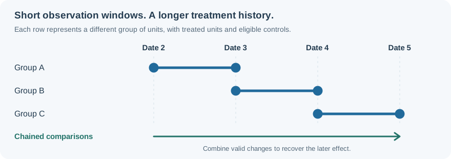
For each window, compare the outcome change of treated units with the change of suitable controls. Under parallel trends and representative mean changes, the first comparison identifies the effect at date 3. The next identifies how that effect changes between dates 3 and 4; the final comparison supplies the next increment. Their sum recovers the effect at date 5.
The units do not need identical individual changes. What matters is that each comparison represents the relevant cohort and control populations. When several valid comparisons inform the same effect, cdid combines them by generalized method of moments, accounting for their covariance.
The rotating-panel example makes this concrete: 1,000 units, five dates, two observed outcomes per unit, and zero complete cases. Chaining recovers all three requested posttreatment effects. With true effects of 1.00, 1.25, and 1.50, the recorded estimates are 0.895, 1.202, and 1.350, with analytical standard errors of 0.092, 0.125, and 0.157.
Why changing composition need not erase identification
Incomplete panels raise a second issue: the units observed at one date can differ systematically from those observed at another. Comparing their average outcome levels can then mix treatment effects with changes in sample composition.
Within-unit differences remove stable unit effects. A persistently high outcome level disappears when we subtract one observation of that unit from another. This permits observation to depend on an unobserved fixed component, provided that selection does not also distort the mean changes needed for the analysis.
The guide’s changing-composition example follows this idea. Each unit is observed at two consecutive dates. Treated units with high fixed outcomes tend to appear early; those with low fixed outcomes appear late. The true treatment effect is 1 at every posttreatment date. In this design, the population comparisons are:
| Period | True effect | Chained comparisons | Comparisons of observed levels |
|---|---|---|---|
| 3 | 1.00 | 1.00 | 0.60 |
| 4 | 1.00 | 1.00 | 0.20 |
| 5 | 1.00 | 1.00 | 0.00 |
These are population calculations, rather than fitted estimates. They show why observation that selects outcome levels can still leave useful changes. In the recorded sample, the date-5 chained estimate is 0.868; the observed-level estimate is −0.063.
The distinction is substantive. If the stable component also predicts untreated trends or treatment-effect heterogeneity, removing it from levels does not automatically remove selection in changes. Conversely, when each date’s observed sample represents the population, comparisons of levels can be valid too.
Flexible adjustment across treatment cohorts
The package estimates ATT(g,t): the average effect at date t for units first treated at date g. This allows staggered adoption and effects that differ by cohort and time since treatment. Researchers can choose never treated or not yet treated controls and adjust for covariates through IPW, OR, or DR.
In the treatment-choice example, 2,000 units are followed over six dates, with two treatment cohorts, incomplete outcomes, and treatment assignment related to a covariate. All three approaches track the known event-time pattern:
| Time since treatment | True effect | IPW | OR | DR |
|---|---|---|---|---|
| 0 | 1.00 | 1.028 | 1.032 | 1.026 |
| 1 | 1.25 | 1.240 | 1.230 | 1.238 |
| 2 | 1.50 | 1.538 | 1.530 | 1.528 |
| 3 | 1.75 | 1.744 | 1.724 | 1.729 |
The columns are estimates from the same generated panel. Their agreement illustrates how several treatment adjustments fit within one chained framework; it does not require choosing a different target or discarding incomplete histories.
Correcting for who gets observed
Treatment adjustment and missing-outcome adjustment answer different questions. A treatment propensity model helps make a cohort comparable with controls. An observation model helps make the changes we observe representative of the population we want to study. Addressing one does not automatically address the other.
When measured covariates explain selection in mean changes, selection = "conditional_mtar" enables three approaches:
- Observation weighting: reweight observed changes by their probability of being observed at both dates.
- Change imputation: model actual changes, including treatment effects, and predict them for the study population.
- Augmented correction: combine change predictions with weighted prediction errors from observed units.
The change-imputation example compares these approaches on one incomplete panel where their required models are correctly specified. The recorded average-effect estimates are 1.624 with weighting, 1.629 with imputation, and 1.629 with augmentation, each with a standard error near 0.038. The known average effect for the generated treated units is 1.627.
Treatment DR combined with the augmented correction provides robustness in both layers. Either the treatment propensity or counterfactual regression must be correct, and either the observation or actual-change model must be correct, with the other identification and regularity conditions maintained. The model-robustness guide explains these alternatives and distinguishes theoretical guarantees from executed examples.
More information when stronger assumptions are credible
By default, PT-post imposes parallel trends from each cohort’s reference period onward. PT-all adds restrictions from a chosen common start date. These additional restrictions can make more effects available or improve precision when they are credible.
The PT-all walkthrough compares both choices on the same incomplete panel, then introduces an earlier untreated outcome pulse that violates the stronger assumption. It shows why choosing restrictions is an economic judgment: additional information is useful only when the assumptions that justify it hold. The start date should be chosen on substantive grounds before inspecting results.
Chaining can also improve precision relative to level comparisons by removing persistent differences between units. The size of that gain depends on outcome persistence, the observation windows, and the covariance of the comparisons. The precision guide explains the trade-offs.
The numerical examples above are recorded runs from October 29, 2026, using cdid 1.1.0.0, did 2.5.1, and DRDID 1.3.0 under R 4.5.2. The OR/DR examples retain their historical pooled outcome specification; the current default fits separate comparison regressions. Together, the examples demonstrate useful behavior across distinct designs. They do not establish repeated-sample bias, coverage, or a universal precision advantage for the current release.
A familiar R workflow
Getting started requires a standard R installation:
install.packages("cdid")
library(cdid)
vignette("cdid", package = "cdid")
Estimate cohort and period effects with cdid::att_gt(), aggregate them with cdid::aggte(), and plot them with cdid::ggdid(). The package supports event-time, cohort, calendar, and overall summaries, analytical or multiplier inference, clustering, simultaneous bands, and pretrend tests. tidy() and glance() expose results and support diagnostics. Ordinary mode delegates to did, including for repeated cross sections.
For incomplete panels, keep missing outcomes as NA. Define the study population with a unit table supplied through frame when needed, rather than allowing complete-case selection to define it implicitly. Inspect which effects are supported: a chain needs valid comparisons, adequate overlap, and the relevant missingness assumptions. Unsupported effects are reported with a reason.
Visit the updated project page for an overview, the full guide for methods and examples, and the practical notebook to explore the workflow on a configurable synthetic panel. Source code and issue reporting are on GitHub.
Bellégo, C., Benatia, D., and Dortet-Bernadet, V. (2025). The Chained Difference-in-Differences. Journal of Econometrics, 248, article 105783.